ASE Tutorials

Transition State and Free Energy Calculations

In this final exercise, you will be calculating the transition state energy for N₂ dissociation using the fixed bond length (FBL) method. The nudged elastic band (NEB) method can more accurately determine the saddle point for the transition state, but it is more computationally intensive and we won’t be using it for this course. You will also be calculating the vibrational modes for the adsorbed species and using the modules within ASE to determine free energies. Finally, you will be putting everything together in order to calculate the reaction rate.

Fixed Bond Length Calculation
Vibrational Frequencies and Free Energies
Reaction Rate
Nudged Elastic Band Calculation (Optional)

Required Files

Obtain the required files by running:

on Sherlock:

cd $SCRATCH
wget http://chemeng444.github.io/ASE/Transition_States/exercise_3_sherlock.tar
tar -xvf exercise_3_sherlock.tar

or on CEES:

cd ~/$USER
wget http://chemeng444.github.io/ASE/Transition_States/exercise_3_cees.tar
tar -xvf exercise_3_cees.tar

This will create a folder called Exercise_3_Transition_States.

Fixed Bond Length Calculation

The fixed bond length (FBL) method is a much faster but cruder way to approximate the minimum energy path and determine the transition state energy. It doesn’t require parallelization over different nodes but may not give you the exact transition state. Generally, one could perform a fixed bond length calculation first and determine if a transition state was found (by checking the vibrational modes). If the transition state is poorly described, then a NEB calculation can be performed based on the fixed bond length results as the inputs.

In a FBL calculation, you provide an initial state, then, you iteratively decrease the distance between the two atoms and optimize the geometry of the entire structure while keeping the bond length fixed. This will approximate the minimum energy pathway (MEP) between the initial and final states. Since we are iteratively decreasing the distance, our input in this case would correspond to the final state in our N₂ dissociation reaction. We then fix the bond length between the two N* atoms that are required to come together and form a bond. We are thus calculating the reverse reaction: 2N* → N₂ + 2*. Follow the fbl.py script to determine the transition state for the dissociative adsorption of N₂ on your metal. The script requires an initial state and a specification of the two atoms whose distance is to be fixed (the two N* atoms).

When deciding which of your 2N* states to include, you should consider all fully dissociated states within 0.5 eV of the lowest energy configuration, to ensure that you have found the lowest possible barrier. Note that we want to find the barrier for N₂ dissociation, so any configuration you found that is not dissociated (N₂* rather than 2N*) should be ignored.

atom1=12
atom2=13

Make sure that the two atoms whose bond distance is to be fixed is correct. Since FixBondLength() is a constraint, all constraints on the unit cell must be re-specified when setting the constraints. For surfaces:

constraints = [FixBondLength(atom1,atom2)]
mask = [atom.z < 10 for atom in atoms]      # atoms in the structure to be fixed
constraints.append(FixAtoms(mask=mask))
atoms.set_constraint(constraints)

or for clusters:

fixatoms = FixAtoms(indices=[atom.index for atom in atoms if atom.symbol in metals])
constraints.append(fixatoms)

Then for each fixed N-N distance, a structural relaxation is performed.

These settings have already been set for you in the fbl.py script. MAKE SURE TO READ THROUGH THE SCRIPT AND FOLLOW THE INSTRUCTIONS.

To reduce the likelihood of mistakes, we have highlighted the sections needing your input:

#########################################################################################################
#####                                     YOUR SETTINGS HERE                                        #####
#########################################################################################################

Make sure to edit the settings in there!

The fixed bond length calculation can continue beyond the final state and start to give you structures with unrealistically high energies. These would not be relevant for the reaction path and you should select only the trajectory images you want to view. To do this, you can combine the .traj files from each step first,

ase-gui i?.traj i??.traj -n -1 -o combined.traj

where ase-gui will read all files of the form i?.traj followed by i??.traj, combine their final steps (using -n -1), and then write out a combined file called combined.traj.

Then, to select the range of images within combined.traj, you can use the @ symbol followed by a range, such as:

ase-gui combined.traj@:22

which will display images 1 through 22 within the combined trajectory file. The image range follows Python syntax. Choose the range where you get a clear view of the initial state, transition state, and final state. You can use ase-gui to view the reaction coordinate:

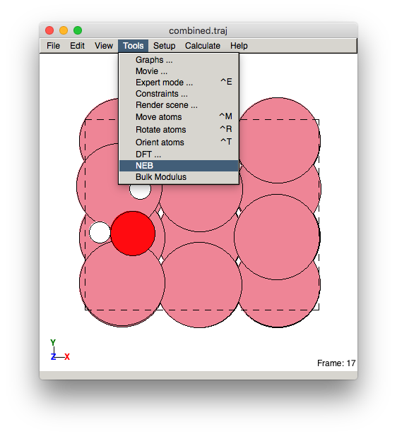
Tools > NEB

Even though the NEB menu option was intended for viewing NEB trajectories, it will work for any transition state calculation. You should see a plot that looks like this:

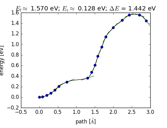
Reaction Coordinate

You should only pay attention to the peak of the plot, which is where the transition state is. The FBL calculation will not necessarily find the final state (in this case, gaseous N₂), so the final state energy in the plot will not generally be correct.

Keep in mind that this plot is a BACKWARDS description of the reaction path for N₂ dissociation. The first image is actually the last step (fully dissociated state).

If the bond length becomes unrealistically short, you will also see large spikes in the total energy towards the end of your calculation. You can safely ignore these images.

Note that on very reactive surfaces, the FBL calculation may not be able to find the desorbed N₂* state before the bond length becomes unrealistically short (the adsorption of N₂* is extremely favorable). This is okay because we would expect the relevant transition state to occur AFTER the adsorption step for such a reactive surface. You can therefore use the transition state calculation as normal in this case even though FBL does not recover the gaseous N₂ state.

Requirement: Turn in an image of the transition state and the reaction coordinate.

Vibrational Frequencies and Free Energies

Calculate the vibrational frequencies for transition state and the final state using the run_freq.py script. See the ASE page for a detailed explanation of how this is implemented. Use ase-gui to view the vibrational modes, which are written out as vib*.traj files. There should be $3N$ vibrational modes for all adsorbed states, and $3N - 1$ vibrational modes for the transition state.

Since the fixed bond-length method cannot guarantee a solution at the saddle point (the image with the highest energy might not be exactly at the transition state), you may encounter multiple imaginary modes when you calculate the vibrational frequencies. In this case, the following scheme can be used:

Any adsorbate should have $3N$ non-imaginary vibrational modes
Transition states should have $3N – 1$ non-imaginary vibrational modes and one imaginary mode
If there are extra imaginary modes replace < 7 meV with 7 meV

For the gas phase species, we will provide the results for N₂, H₂, and NH₃ for you. You calculated the results for N₂ in the last exercise and you can use either your own results or the one provided. These are in the Gaseous_Molecules\ folder.

Requirement: Calculate the vibrational frequencies for:

Initial state: 2N*
Transition state: N-N*
Intermediates: N*, NH*, NH₂*, NH₃*,H*

Reaction Rate

Using the vibrational frequencies associated with initial, final and transition states, evaluate the rate constant of N₂ dissociation on the metal surface and cluster based on harmonic transition state theory (hTST). In addition, evaluate the rate constant based on the Arrhenius relationship by using the free energy associated with the initial, final, and transition states that were directly calculated from ASE Quantum Espresso. For the free energies, use the get_ads_free_energy.py script for adsorbed states and get_gas_free_energy.py for N₂.

To calculate the rate of N₂ dissociation, one can assume that the first step is rate determining and all other steps are in equilibrium. This leads to two reactions:

$\begin{align} &(1) \quad &\mathrm{N_2} + 2* \rightarrow \mathrm{2N}*\\ &(2) \quad &\mathrm{N}* + \frac{3}{2}\mathrm{H}_{2\,\mathrm{(g)}} \leftrightarrow \mathrm{NH}_{3\,\mathrm{(g)}} + * \end{align}$

The rate constant and equilibrium constants are:

$k_1 = \frac{k_\mathrm{B} T}{h} \exp\left(-\frac{\Delta G_\mathrm{TS,1}}{k_\mathrm{b}T}\right)$

For the entire reaction:

$K_\mathrm{eq} = \exp\left(-\frac{\Delta G_\mathrm{rxn}}{k_\mathrm{B}T}\right)$

and for only the second reaction:

$K_\mathrm{2} = \exp\left(-\frac{\Delta G_\mathrm{rxn,2}}{k_\mathrm{B}T}\right)$

The reaction rate (turnover frequency, TOF) for the entire reaction is then given in a simply analytical form:

$\mathrm{TOF} = k_1 P_\mathrm{N_2} \left(1+\frac{P_\mathrm{NH_3}}{K_2 P_\mathrm{H_2}^{1.5}}\right)^{-2}\left(1 - \frac{P_\mathrm{NH_3}^2}{K_\mathrm{eq}P_\mathrm{H_2}^3 P_\mathrm{N_2}}\right)$

Requirement:

Plot the log of the rate constant versus the inverse temperature.

Nudged Elastic Band Calculation (Optional)

To perform a nudged elastic band (NEB) calculation, one needs to provide an initial and final state trajectory. A series of “images” between the initial and final states will then be used to determine the minimum energy path. This band of images will be relaxed. For a NEB calculation, you only need to provide the initial and final state and the number of images in between. Go through the neb.py script. Typically 5~7 images between the initial and final states will be sufficient. Intermediate images will be generated using a linear interpretation of the initial and final trajectory. An odd number of images should be chosen so that the one image will be at the transition state. NEB calculations can take a long time, and the neb_restart.py should be used to read in the previous images. You can also start at with k-points to speed up the calculation, and then restart the calculation with higher k-points.

In the neb.py file make sure the line specifying the number of nodes.

#SBATCH --nodes=5

corresponds to the number of intermediate images. Check that intermediate_images = 5 matches.

Both neb.py and neb_restart.py scripts require the initial and final states of the reaction path to be provided. This is specified in the lines:

initial = io.read('neb0.traj')
final = io.read('neb6.traj')

make sure that the trajectory files are in the directory and are named in the same manner. For the neb_restart.py script, the initial and final trajectories must be named in the neb*.traj format, where * is a number. The script will read in all intermediate images based on the number in the initial and final trajectory.

To view all the trajectory files, run the following command

ase-gui neb*.traj –n -1

where all files of the form neb*.traj (with * referring to any number of characters) will be opened in ag. The -n flag specifies the image within each trajectory file. Since you are optimizing the entire reaction path, each step in the NEB will be stored in each image file. Specifying -n -1 tells ase-gui to only read the last image of each file (i.e. the most current step).